permutation_lm
permutation_lm.RdPerforms a permutation test on a dataset (dataframe) testing if the more complicated of two linear models (linear, quadratic or cubic) fits the data significantly better than the less complicated model. It prints a permutation-plot with the permuted null-distribution and the observed value (simple or nice depending on choice) and gives a p-value.
permutation_lm(dataset, predictor, response, model1, model2, no_perm, plot, gg_plot)
Arguments
| dataset | the dataset containing the data you want to test in the form of a data frame – the data needs to contain (at least) a column with the names of the two groups you want to test against each other and a column with the values of the different cases for these groups. |
|---|---|
| predictor | the name of the column with predictor values (string) |
| response | the name of the column with response values (string) |
| model1 | the name of one of the models you want to test (string), possible values: “linear”, “quadratic” or “cubic” |
| model2 | the name of the other model you want to test (string), possible values: “linear”, “quadratic” or “cubic” |
| no_perm | the number of permutations to make, default=10000 |
| plot | whether or not you want it to plot the distribution of the permutation at all, default=T |
| gg_plot | a logic value indicating whether a nice ggplot plot should be printed (requires ggplot2), default=F (as opposed to a simple plot) |
| progress | a logic value indicating whether a progress bar should be printed, default=T |
Details
The calculations that are done in this function are an anova of the chosen two models of the dataset, giving a value from the F-distribution. The two models are made, depending on which models are chosen, using the build-in lm() function. The F-value calculated will be the observed value. The dataset values are then randomly shuffled, the two models are made again, and the F-value is calculated and saved – this is done as many times as the no_perm is defined as. This will give a “new F-distribution”, that will be our null-distribution, where a p-value then can be calculated as the amount of times the value of the permuted values are bigger or equal to the value of the observed + 1, divided by the total amount of permutations + 1:
$$p_{val} = (\sum(perm_{val} \ge observed)+1) / (\#permutation+1)$$
We add one as a precaution, since we do not know the value of the next permutation and thereby always should expect the “next” value to be at least as extreme as the observed. If this value is below the chosen significance value, the more complicated of the two models chosen will be significantly better than the less complicated of the two models.
Value
permutation_lm returns a list with the class “htest” containing the following:
the method of the test
the p-value of the test
the value of the observed F-value for the models
the names of the predictor and response tested
Examples
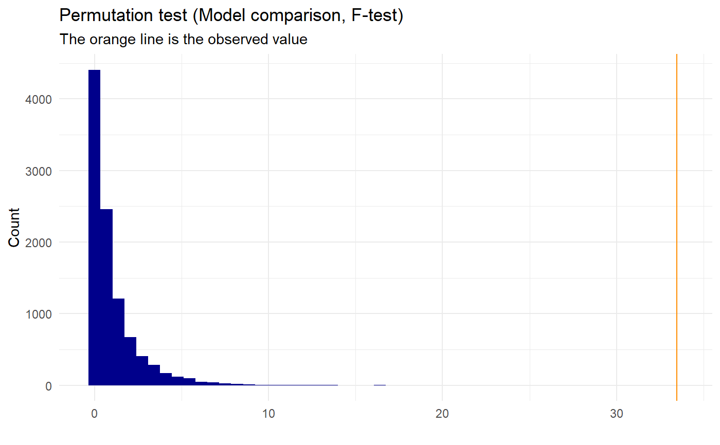
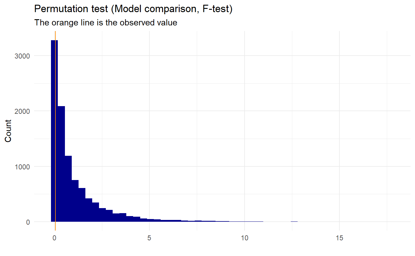
set.seed(0) x <- sample(c(-10:10), 100, replace=T) y <- 4*x^2+3+50*sample(c(-10:10), 100, replace=T) data <- data.frame(x,y) permutation_lm(data, "x","y","quadratic", "linear", plot=TRUE, gg_plot=TRUE, progress=FALSE)#> #> Permutation Test (ANOVA) for quadratic and linear models #> #> data: Permutation for predictor x and response y #> p-value = 9.999e-05 #> sample estimates: #> Observed F value between models #> 33.45256 #>permutation_lm(data, "x","y","cubic","quadratic", plot=TRUE, gg_plot=TRUE, progress=FALSE)#> #> Permutation Test (ANOVA) for cubic and quadratic models #> #> data: Permutation for predictor x and response y #> p-value = 0.8302 #> sample estimates: #> Observed F value between models #> 0.04548759 #>